When Multiphysics Met Robotics: The Failed Prints That Defined Our Roadmap

The cleanest engineering diagrams usually appear after the messiest experiments.

Our first attempts to connect robotic deposition with multiphysics did not begin as a polished software architecture. They began with overheated material, unstable process parameters, disconnected tools and a growing collection of data that did not yet share one timeline.

Those problems became the design brief for QH Build.

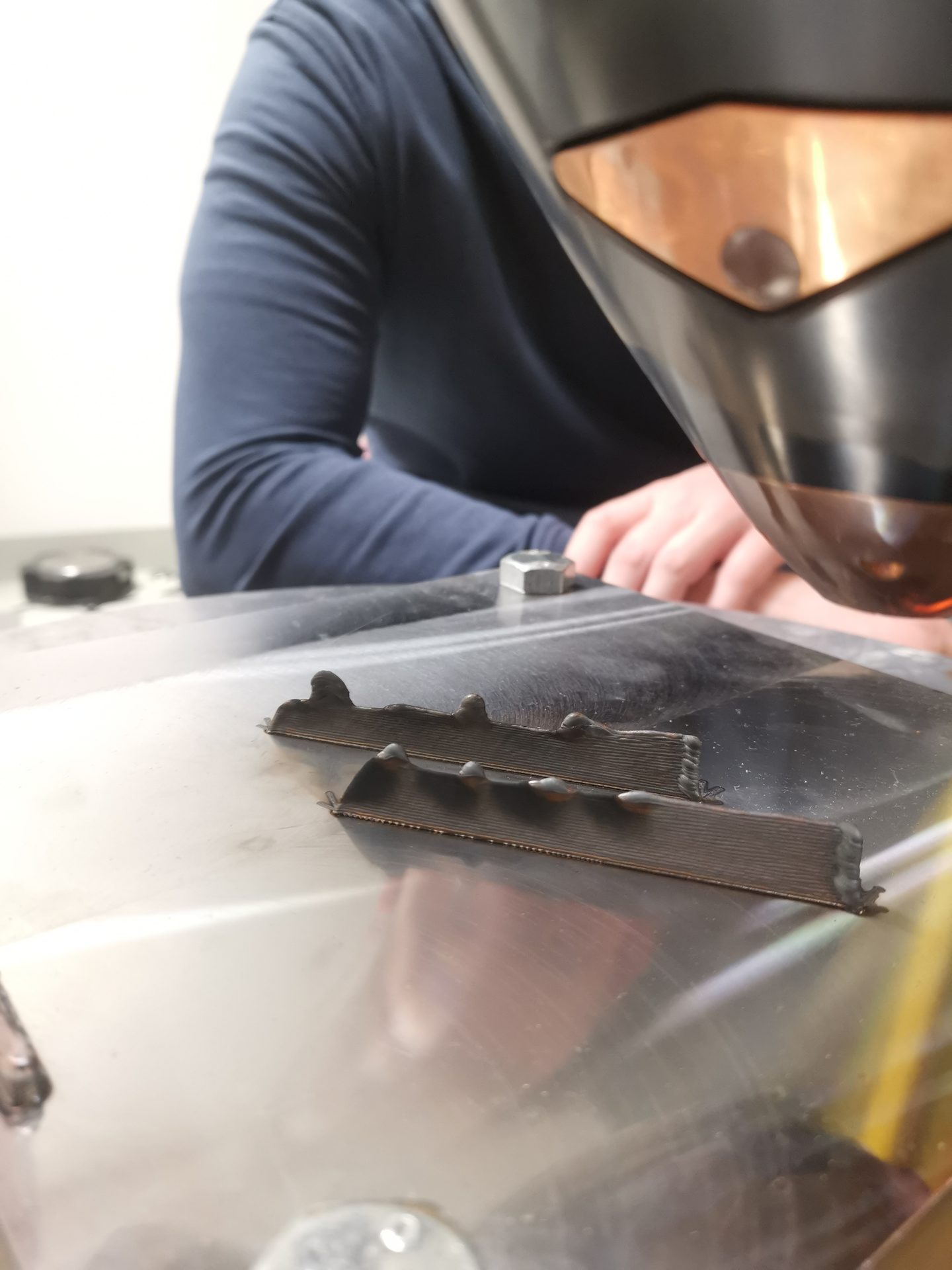
An early print affected by overheating and unsuitable process parameters

Problem one: a valid robot path can still create a failed process

The robot knew where to move. The deposition head knew when to deliver energy and material. The CAM system showed a plausible geometry.

Yet the first physical results made the missing information visible. A toolpath can be kinematically valid while the thermal process is unstable. The robot may slow down near a transition, but the laser power or wire feed may remain unchanged. Energy and material then accumulate in a smaller region. The result can be overheating, excessive bead growth or a local defect.

From the robotics side, the path was correct. From the physics side, the boundary conditions had changed. Neither tool alone described the complete event.

Problem two: the robotics and physics models were disconnected

The next question was not simply “Which laser power should we use?” It was “Which laser power should we use at this real speed, on this trajectory, with this start delay, standoff distance and thermal history?”

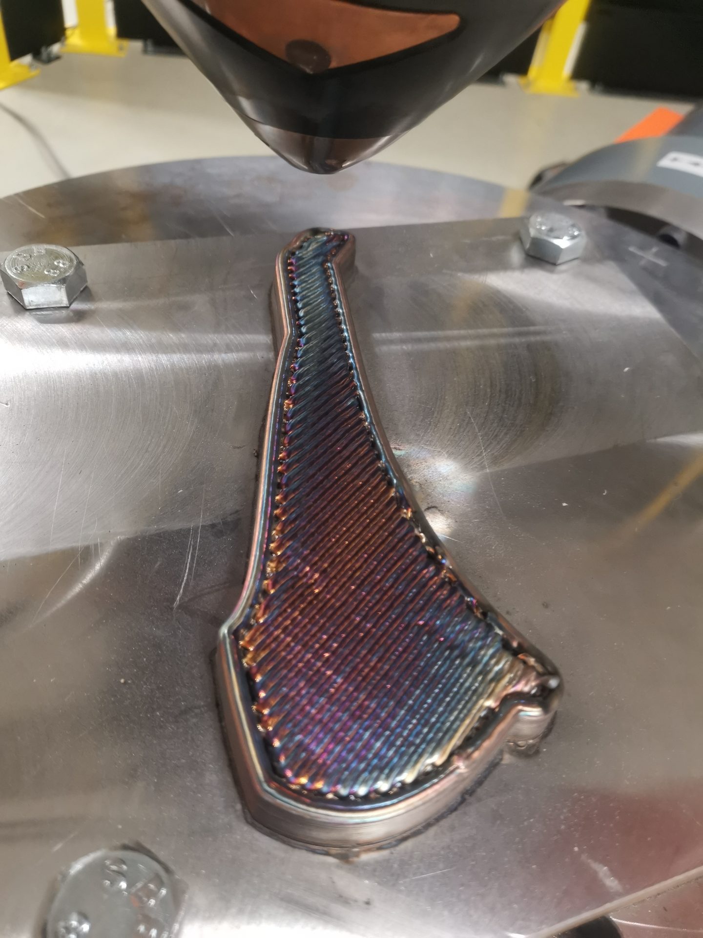A deposited part illustrating the disconnect between robotic planning and process physics

Traditional development often sends information in one direction. A path is exported from CAM, simplified and then used as an input to a process simulation. If the physical build fails, an engineer manually changes parameters and starts again.

We needed a shared representation in which robot motion and process physics could influence the same evolving part.

Problem three: trial and error does not scale

The immediate response to an unstable process is usually to print more test samples. Vary power. Vary speed. Vary wire feed. Change standoff distance. Repeat.

That work is necessary, especially when establishing a new material or machine. The problem is combinatorics. Five parameters with only five candidate values already create 3,125 combinations. Add path curvature, orientation, layer history and external-axis motion, and a parameter table becomes unmanageable.

Our early test matrix was valuable because it created empirical evidence. It was also a clear demonstration of why physical experiments must be guided by simulation.

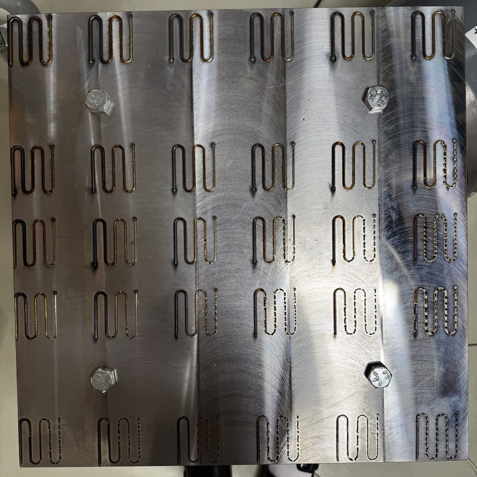A matrix of physical parameter tests used during early process development

The objective is not to remove experiments. It is to stop using expensive machine time to test combinations that a model could reject in advance.

The turning point: log the real machine

A digital twin cannot be calibrated from nominal values alone. We therefore began logging the robot and process data.

The robot stream included positions, velocities, axis states and controller events. This made it possible to see what the machine executed rather than what the program commanded.

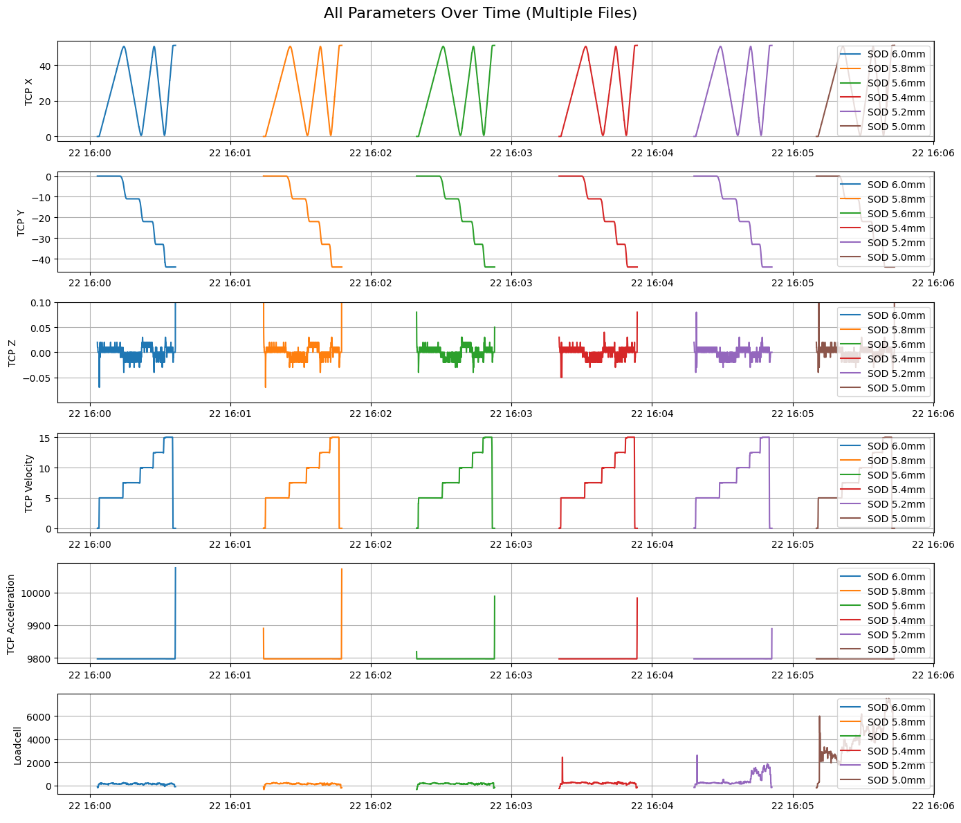Robot parameters logged in real time across repeated tests

The process stream added another layer: deposition states, sensor signals and near-real-time manufacturing data. Once these signals could be aligned, the connection between motion and material response became measurable.

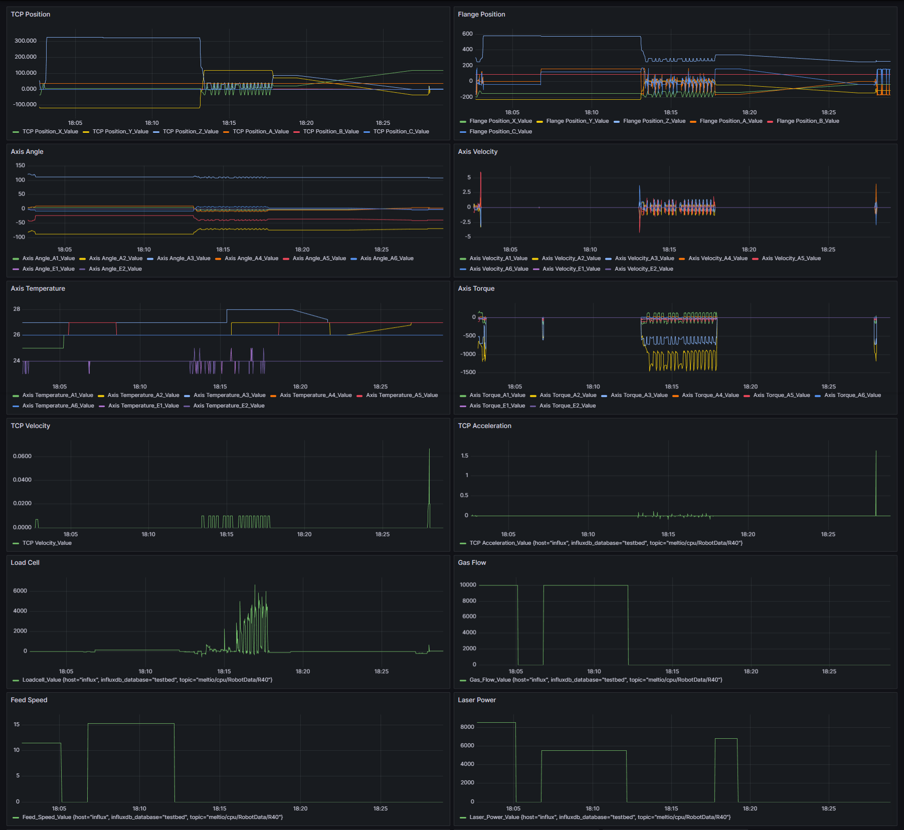Near-real-time process and sensor data collected from the manufacturing system

This changed the question from “Why did this part fail?” to a more useful sequence:

• What did the controller do at the defect location?
• What process commands were active?
• How much material and energy were delivered?
• What had already been deposited underneath?
• What did the thermal and fluid model predict?
• Did the physical measurements confirm the prediction?

The architecture that emerged

These experiments led directly to the separation of responsibilities in our platform.

The Kinematic and Dynamic Deposition Model handles the fast, controller-aware layer. It tracks the robot, external axes, deposition timing and geometric material accumulation. It can quickly identify locations where motion blending, deceleration or start-stop timing may cause over- or under-deposition.

The Multiphysics Deposition Model receives the relevant motion and process history and resolves the material behaviour: energy absorption, melt-pool flow, surface tension, phase change and thermal history.

The synchronized data layer connects both models to physical evidence.

What industry can learn from our failures

Early failed prints are not wasted when they are converted into structured data. They become calibration cases, validation cases and process boundaries.

For a production team, this approach can reduce commissioning time in several ways:

• use fast simulation to eliminate poor paths and timing strategies;
• reserve high-fidelity simulation for the most critical regions;
• run physical tests where they create the most information;
• record every test in a format that can be replayed and compared;
• reuse calibrated process knowledge when moving to a new geometry.

Our roadmap was not invented in isolation. It was shaped by the exact moments when the existing workflow failed.

That is still how we develop: observe the gap, instrument it, model it, validate it and turn it into a repeatable tool.